Analysis of Slide-seqV2 mouse olfactory bulb dataset#
In this tutorial, we demonstrate SpaMetric on the analysis of Slide-seqV2 mouse olfactory bulb dataset including
Spatial reconstruction
Mini-batch metric learning
Spatial domain identification
Finding differentially expressed genes
Spatial domain annotation
The dataset is available at Single Cell Portal (Puck_200127_15).
[1]:
import numpy as np
import pandas as pd
import scanpy as sc
import matplotlib.pyplot as plt
import seaborn as sns

import SpaMetric as spm
Data loading and preprocessing#
We load the dataset and find top 8000 highly variable genes.
[2]:
adata = sc.read_h5ad('./data/Puck_200127_15.h5ad')
adata
[2]:
AnnData object with n_obs × n_vars = 21724 × 21220
    obsm: 'spatial'
[3]:
sc.pp.highly_variable_genes(adata, n_top_genes=8000, flavor='seurat_v3')
Spatial reconstruction#
We perform spatial reconstruction to aggregate expression from spatial neighbors.
[4]:
spm.spatial_reconstruction(adata, n_neighbors=30)
Mini-batch metric learning#
We select 4000 reference centers and then perform mini-batch metric learning on the reconstructed data.
[5]:
sc.pp.pca(adata)
spm.reference_centers(adata, n_centers=4000)
C:\ProgramData\Anaconda3\lib\site-packages\sklearn\cluster\_kmeans.py:887: UserWarning: MiniBatchKMeans is known to have a memory leak on Windows with MKL, when there are less chunks than available threads. You can prevent it by setting batch_size >= 4096 or by setting the environment variable OMP_NUM_THREADS=1
  warnings.warn(
Since this step takes some time, we load previouly computed AnnData.
[6]:
# spm.metric_learning_minibatch(adata)

adata = sc.read_h5ad('./data/Puck_200127_15_results.h5ad')
adata
[6]:
AnnData object with n_obs × n_vars = 21724 × 21220
    obs: 'reference_centers'
    var: 'highly_variable', 'highly_variable_rank', 'means', 'variances', 'variances_norm'
    uns: 'hvg', 'metric', 'pca', 'reference_centers', 'spatial_reconstruction'
    obsm: 'X_pca', 'metric', 'spatial'
    varm: 'PCs'
    layers: 'counts', 'log1p'
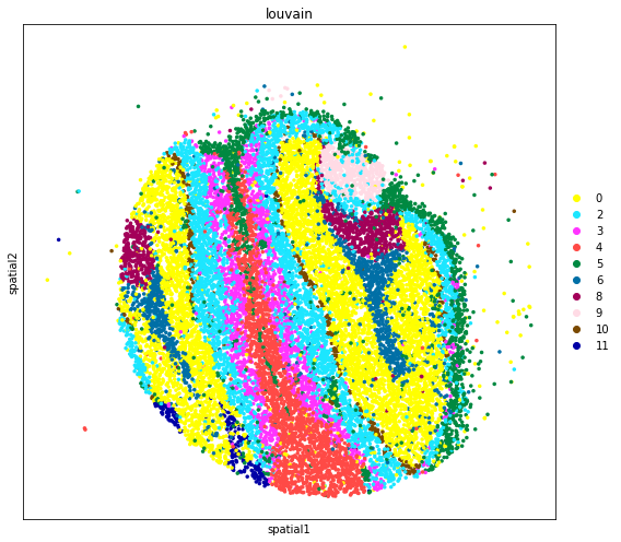
Spatial domain identification#
We create a temporary AnnData using the sample-by-reference metric matrix and then interoperate with SCANPY to identify spatial domains.
[7]:
adata_V = sc.AnnData(adata.obsm['metric'])
adata_V.obs_names = adata.obs_names
adata_V.obsm['spatial'] = adata.obsm['spatial']
adata_V
[7]:
AnnData object with n_obs × n_vars = 21724 × 3933
    obsm: 'spatial'
[8]:
sc.pp.pca(adata_V)
sc.pp.neighbors(adata_V)
sc.tl.louvain(adata_V, resolution=0.4)
[9]:
adata.obs['louvain'] = adata_V.obs['louvain']
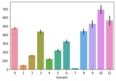
We exclude domain 1 and 7 from downstream analysis, since their average counts are lower than 100.
[10]:
sns.barplot(y=np.sum(adata.layers['counts'].toarray(), axis=1), x=adata.obs['louvain'])
[10]:
<AxesSubplot:xlabel='louvain'>
[11]:
adata_subset = adata[~adata.obs['louvain'].isin(['1', '7']),:]
[12]:
fig, axs = plt.subplots(figsize=(8, 7))

sc.pl.embedding(
    adata_subset,
    basis='spatial',
    color='louvain',
    size=50,
    palette=sc.pl.palettes.default_102,
    legend_loc='right margin',
    show=False,
    ax=axs,
)

plt.tight_layout()
Trying to set attribute `.uns` of view, copying.
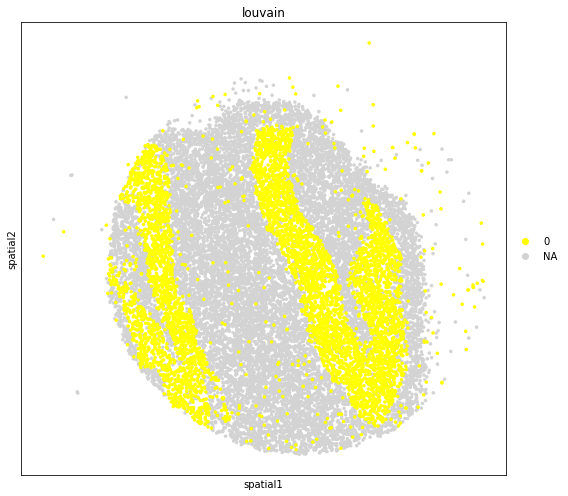
Finding differentially expressed genes#
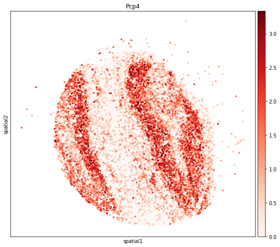
We find the differentially expressed (DE) genes across identified domains and show the domains and their DE gene expression patterns in spatial coordinates.
[13]:
sc.tl.rank_genes_groups(adata_subset, groupby='louvain', use_raw=False, layer='counts', method='t-test_overestim_var')
[14]:
de_genes = pd.DataFrame(adata_subset.uns['rank_genes_groups']['names']).iloc[:10,:]
de_genes
[14]:
| 0 | 2 | 3 | 4 | 5 | 6 | 8 | 9 | 10 | 11 | |
|---|---|---|---|---|---|---|---|---|---|---|
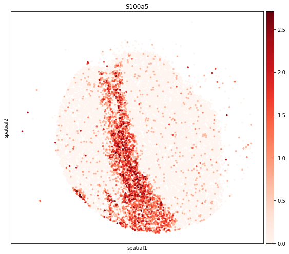
| 0 | Pcp4 | mt-Nd4 | Nrsn1 | S100a5 | Ptgds | Mbp | Cpne6 | Gap43 | Rab3b | S100a5 |
| 1 | Camk2n1 | Doc2g | Cck | Fabp7 | Hbb-bs | Plp1 | Hap1 | Snca | Doc2g | Omp |
| 2 | Pcp4l1 | mt-Nd1 | S100a5 | Apod | Hba-a1 | Mobp | Macrod2 | Doc2g | Map1b | Stoml3 |
| 3 | Camk2b | mt-Cytb | mt-Cytb | Gng13 | Hbb-bt | Cnp | Nos1 | Uchl1 | Slc17a7 | Atf5 |
| 4 | Meis2 | mt-Rnr1 | Calb2 | Omp | Igf2 | Mal | Synpr | Fxyd6 | Atp1b1 | Scgb1c1 |
| 5 | Calm2 | mt-Nd2 | Olfm1 | Atf5 | Hba-a2 | Cldn11 | Tac1 | Stmn2 | Olfm1 | Vmo1 |
| 6 | Gng4 | mt-Nd5 | mt-Nd1 | Npy | Mgp | Fth1 | Pnmal2 | Calb2 | Syp | Cbr2 |
| 7 | Malat1 | mt-Co1 | mt-Nd4 | Ptn | Aebp1 | Trf | Atp2b4 | Rasgrp1 | Stmn3 | Tmsb4x |
| 8 | Nrxn3 | mt-Rnr2 | Trh | Kctd12 | Col1a2 | Mog | Nrxn3 | Tuba1a | Thy1 | Gng13 |
| 9 | Ppp3ca | Slc6a11 | Sparcl1 | Stoml3 | Slc6a20a | Mag | Necab2 | Map1b | Shisa3 | Calm1 |
[15]:
fig, axs = plt.subplots(figsize=(8, 7))

sc.pl.embedding(
    adata_subset,
    basis='spatial',
    color='louvain',
    groups='0',
    layer='log1p',
    size=50,
    palette=sc.pl.palettes.default_102,
    legend_loc='right margin',
    show=False,
    ax=axs,
)

plt.tight_layout()
[16]:
fig, axs = plt.subplots(figsize=(8, 7))

sc.pl.embedding(
    adata_subset,
    basis='spatial',
    color=de_genes.iloc[0,0],
    layer='log1p',
    size=50,
    color_map='Reds',
    vmax='p99.9',
    show=False,
    ax=axs,
)

plt.tight_layout()
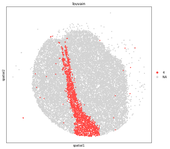
[17]:
fig, axs = plt.subplots(figsize=(8, 7))

sc.pl.embedding(
    adata_subset,
    basis='spatial',
    color='louvain',
    groups='4',
    layer='log1p',
    size=50,
    palette=sc.pl.palettes.default_102,
    legend_loc='right margin',
    show=False,
    ax=axs,
)

plt.tight_layout()
[18]:
fig, axs = plt.subplots(figsize=(8, 7))

sc.pl.embedding(
    adata_subset,
    basis='spatial',
    color=de_genes.iloc[0,3],
    layer='log1p',
    size=50,
    color_map='Reds',
    vmax='p99.9',
    show=False,
    ax=axs,
)

plt.tight_layout()
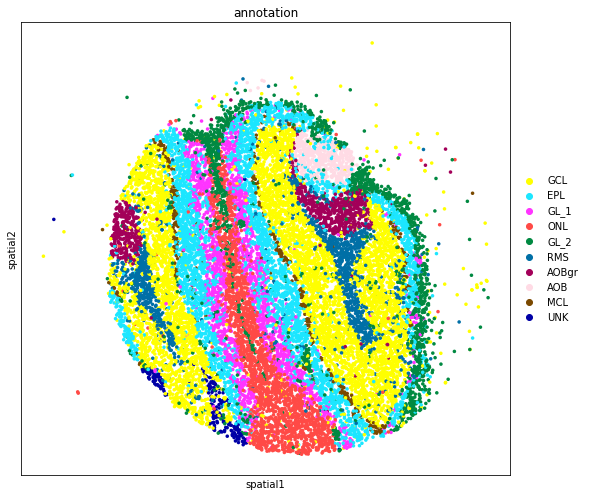
Spatial domain annotation#
We annotate the spatial domains based on the anatomical annotation from Allen Reference Atlas and marker genes.
[19]:
map_dict = {
    '0': 'GCL',
    '2': 'EPL',
    '3': 'GL_1',
    '4': 'ONL',
    '5': 'GL_2',
    '6': 'RMS',
    '8': 'AOBgr',
    '9': 'AOB',
    '10': 'MCL',
    '11': 'UNK',
}
[20]:
adata_subset.obs['annotation'] = adata_subset.obs['louvain'].map(map_dict).astype('category')
[21]:
fig, axs = plt.subplots(figsize=(8.3, 7))

sc.pl.embedding(
    adata_subset,
    basis='spatial',
    color='annotation',
    size=50,
    palette=sc.pl.palettes.default_102,
    legend_loc='right margin',
    show=False,
    ax=axs,
)

plt.tight_layout()