Analysis of 10x Visium human breast cancer slice

In this tutorial, we demonstrate SpaMetric on the analysis of 10x Visium human breast cancer (block A section 1) slice including

• Spatial reconstruction

• Metric learning

• Spatial domain identification

• Spatial domain annotation

• Finding differentially expressed genes

The dataset is available at 10x genomics website (Spatial Gene Expression >> Visium Demonstration (v1 Chemistry) >> Space Ranger 1.0.0 >> Human Breast Cancer (Block A Section 1)).

import numpy as np
import pandas as pd
import scanpy as sc
import matplotlib.pyplot as plt

import SpaMetric as spm

Data loading and preprocessing

We load the dataset and find top 2000 highly variable genes.

adata = sc.read_visium('./data/Human Breast Cancer (Block A Section 1)/')
adata.var_names_make_unique()
adata

Variable names are not unique. To make them unique, call `.var_names_make_unique`.
Variable names are not unique. To make them unique, call `.var_names_make_unique`.

AnnData object with n_obs × n_vars = 3813 × 33538
    obs: 'in_tissue', 'array_row', 'array_col'
    var: 'gene_ids', 'feature_types', 'genome'
    uns: 'spatial'
    obsm: 'spatial'

sc.pp.highly_variable_genes(adata, n_top_genes=2000, flavor='seurat_v3')

Spatial reconstruction

We perform spatial reconstruction to aggregate expression from spatial neighbors.

spm.spatial_reconstruction(adata)

Metric learning

We perform metric learning on the reconstructed data.

spm.metric_learning(adata)

 83%|█████████████████████████████████████████▎        | 826/1000 [04:14<00:53,  3.25it/s, err=9.73943e-06, converged!]

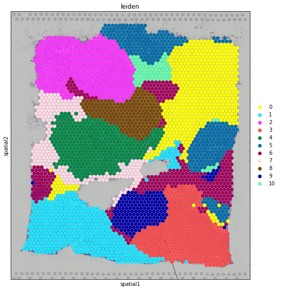
Spatial domain identification

We identify spatial domians using the metric matrix.

sc.tl.leiden(adata, resolution=1.5, neighbors_key='metric')

fig, axs = plt.subplots(figsize=(8, 8))

sc.pl.spatial(
    adata,
    img_key='hires',
    color='leiden',
    size=1.5,
    palette=sc.pl.palettes.default_102,
    legend_loc='right margin',
    show=False,
    ax=axs,
)

plt.tight_layout()

... storing 'feature_types' as categorical
... storing 'genome' as categorical

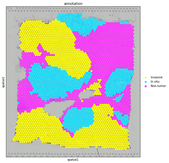
Spatial domain annotation

We annotate the spatial domains based on the pathologist annotation from Fu, H. et al.

map_dict = {
    '0': 'Non-tumor',
    '1': 'Invasive',
    '2': 'Invasive',
    '3': 'Invasive',
    '4': 'In situ',
    '5': 'In situ',
    '6': 'Non-tumor',
    '7': 'Non-tumor',
    '8': 'Invasive',
    '9': 'In situ',
    '10': 'Non-tumor',
}

adata.obs['annotation'] = pd.Categorical(
    adata.obs['leiden'].map(map_dict),
    categories=['Invasive', 'In situ', 'Non-tumor']
)

fig, axs = plt.subplots(figsize=(8, 8))

sc.pl.spatial(
    adata,
    img_key='hires',
    color='annotation',
    size=1.5,
    palette=sc.pl.palettes.default_102,
    legend_loc='right margin',
    show=False,
    ax=axs,
)

plt.tight_layout()

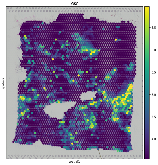
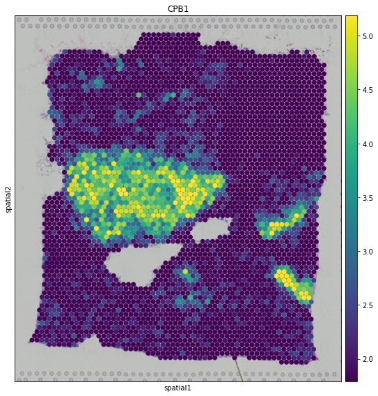
Finding differentially expressed genes

We find the differentially expressed (DE) genes across identified domains and show their expression patterns in spatial coordinates.

sc.tl.rank_genes_groups(adata, groupby='leiden', use_raw=False, layer='counts', method='t-test')

de_genes = pd.DataFrame(adata.uns['rank_genes_groups']['names']).iloc[:10,:]
de_genes

	0	1	2	3	4	5	6	7	8	9	10
0	ACKR1	CXCL14	COX6C	CRISP3	CPB1	MGP	IGKC	C1QA	LINC00645	IFT122	ALB
1	CCL21	CCND1	SNCG	SLITRK6	HLA-B	S100G	IGLC2	APOE	MUC5B	S100G	MGP
2	TNXB	DEGS1	SLC39A6	S100A13	COX6C	DSP	IGHG1	C1QB	PVALB	AC087379.2	BGN
3	CLDN5	S100A11	WFDC2	IGFBP5	IL6ST	TFF1	IGHG3	FABP4	IGFBP2	IFI6	IGHG1
4	CCL19	CPNE7	CSTA	SERHL2	HLA-C	TFF3	C3	GPX3	EXOC2	CALML5	IGFBP7
5	ADAM33	DEGS2	MT-ND1	CALML5	HLA-A	MT-ND3	IGHG4	ADH1B	SLC30A8	HLA-B	COL1A1
6	C7	MUC1	MCCD1	S100A16	ADIRF	RERG	IGLC3	ADIPOQ	COLEC12	HEBP1	SFRP2
7	CHRDL1	RPLP1	RAB11FIP1	KRT8	CFB	STC2	IGHA1	FOLR2	ZNF703	TPD52	CST1
8	ADH1B	PSMB4	MT-CO1	S100A11	B2M	MT-CO1	IGHM	COL14A1	SLC39A6	HLA-A	HTRA3
9	SOD3	RPSA	UGCG	NUPR1	H2AFJ	HK2	TIMP1	HSPB6	AC037198.2	ISG15	COL1A2

fig, axs = plt.subplots(figsize=(8, 8))

sc.pl.spatial(
    adata,
    img_key='hires',
    color=de_genes.iloc[0,4],
    layer='log1p',
    size=1.5,
    palette=sc.pl.palettes.default_102,
    legend_loc='right margin',
    vmin='p50',
    vmax='p99',
    show=False,
    ax=axs,
)

plt.tight_layout()

fig, axs = plt.subplots(figsize=(8, 8))

sc.pl.spatial(
    adata,
    img_key='hires',
    color=de_genes.iloc[0,6],
    layer='log1p',
    size=1.5,
    palette=sc.pl.palettes.default_102,
    legend_loc='right margin',
    vmin='p50',
    vmax='p99',
    show=False,
    ax=axs,
)

plt.tight_layout()