Joint analysis of 10x Visium mouse brain slices

In this tutorial, we demonstrate SpaMetric on the joint analysis of 10x Visium mouse brain serial section 1 (sagittal anterior and posterior) slices including

• Metric learning

• Spatial domain identification

• Spatial subdomain identification

The datasets are available at 10x genomics website (Spatial Gene Expression >> Visium Demonstration (v1 Chemistry) >> Space Ranger 1.1.0 >> Mouse Brain Serial Section 1 (Sagittal-Anterior) & Mouse Brain Serial Section 1 (Sagittal-Posterior)).

We concatenated the images and expression and modified the spatial coordinates to merge two datasets.

import numpy as np
import pandas as pd
import scanpy as sc
import matplotlib.pyplot as plt

import SpaMetric as spm

Data loading and preprocessing

We load the merged dataset and perform preprocessing including finding top 2000 highly variable genes and log transformation.

adata = sc.read_h5ad('./data/Mouse_Brain_Sagittal.h5ad')
adata

AnnData object with n_obs × n_vars = 6050 × 32285
    obs: 'in_tissue', 'array_row', 'array_col', 'batch'
    var: 'gene_ids', 'feature_types', 'genome'
    uns: 'spatial'
    obsm: 'spatial'

sc.pp.highly_variable_genes(adata, n_top_genes=2000, flavor='seurat_v3')
sc.pp.log1p(adata)

Metric learning

We perform metric learning on the preprocessed data.

spm.metric_learning(adata)

 78%|██████████████████████████████████████▉           | 779/1000 [11:40<03:18,  1.11it/s, err=9.92849e-06, converged!]

Spatial domain identification

We identify spatial domians using the metric matrix.

sc.tl.leiden(adata, resolution=3, neighbors_key='metric')

fig, axs = plt.subplots(figsize=(9, 5))

sc.pl.spatial(
    adata,
    img_key='hires',
    color='leiden',
    size=1.5,
    palette=sc.pl.palettes.default_102,
    legend_loc='right margin',
    show=False,
    ax=axs,
)

axs.legend(
    frameon=False,
    loc='center left',
    bbox_to_anchor=(1, 0.5),
    ncol=1,
    fontsize=None,
)

plt.tight_layout()

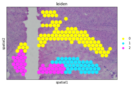
Spatial subdomain identification

We subset the domain of interest and identify subdomains using the metric matrix subset.

adata_subset = adata[adata.obs['leiden']=='16',:]
adata_subset

View of AnnData object with n_obs × n_vars = 174 × 32285
    obs: 'in_tissue', 'array_row', 'array_col', 'batch', 'leiden'
    var: 'gene_ids', 'feature_types', 'genome', 'highly_variable', 'highly_variable_rank', 'means', 'variances', 'variances_norm'
    uns: 'spatial', 'hvg', 'log1p', 'metric', 'leiden', 'leiden_colors'
    obsm: 'spatial'
    obsp: 'metric'

sc.tl.leiden(adata_subset, resolution=0.5, neighbors_key='metric')

Trying to set attribute `.obs` of view, copying.

fig, axs = plt.subplots(figsize=(6, 4))

sc.pl.spatial(
    adata_subset,
    img_key='hires',
    color='leiden',
    size=1.5,
    palette=sc.pl.palettes.default_102,
    legend_loc='right margin',
    show=False,
    ax=axs,
)

plt.tight_layout()