Analysis of 10x Visium invasive ductal carcinoma slice

In this tutorial, we demonstrate SpaMetric on the analysis of 10x Visium invasive ductal carcinoma stained with fluorescent CD3 antibody slice including

• Spatial reconstruction

• Metric learning

• Spatial domain identification

• Spatial domain annotation

• Finding differentially expressed genes

The dataset is available at 10x genomics website (Spatial Gene Expression >> Visium Spatial Gene Expression Fluorescent Demonstration (v1 Chemistry) >> Space Ranger 1.2.0 >> Invasive Ductal Carcinoma Stained With Fluorescent CD3 Antibody).

import numpy as np
import pandas as pd
import scanpy as sc
import matplotlib.pyplot as plt

import SpaMetric as spm

Data loading and preprocessing

We load the dataset and find top 2000 highly variable genes.

adata = sc.read_visium('./data/Invasive Ductal Carcinoma Stained With Fluorescent CD3 Antibody/')
adata.var_names_make_unique()
adata

Variable names are not unique. To make them unique, call `.var_names_make_unique`.
Variable names are not unique. To make them unique, call `.var_names_make_unique`.

AnnData object with n_obs × n_vars = 4727 × 36601
    obs: 'in_tissue', 'array_row', 'array_col'
    var: 'gene_ids', 'feature_types', 'genome'
    uns: 'spatial'
    obsm: 'spatial'

sc.pp.highly_variable_genes(adata, n_top_genes=2000, flavor='seurat_v3')

Spatial reconstruction

We perform spatial reconstruction to aggregate expression from spatial neighbors.

spm.spatial_reconstruction(adata)

Metric learning

We perform metric learning on the reconstructed data.

spm.metric_learning(adata)

 60%|██████████████████████████████                    | 601/1000 [04:34<03:02,  2.19it/s, err=9.86375e-06, converged!]

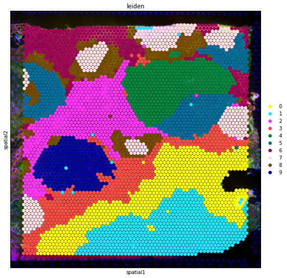
Spatial domain identification

We identify spatial domains using the metric matrix.

sc.tl.leiden(adata, resolution=1.5, neighbors_key='metric')

fig, axs = plt.subplots(figsize=(8, 8))

sc.pl.spatial(
    adata,
    img_key='hires',
    color='leiden',
    size=1.5,
    palette=sc.pl.palettes.default_102,
    legend_loc='right margin',
    show=False,
    ax=axs,
)

plt.tight_layout()

... storing 'feature_types' as categorical
... storing 'genome' as categorical

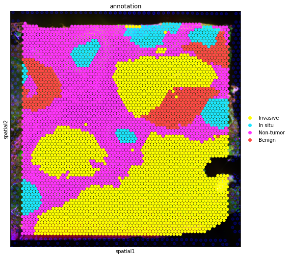
Spatial domain annotation

We annotate the spatial domains based on the pathologist annotation from Zhao, E. et al.

map_dict = {
    '0': 'Invasive',
    '1': 'Invasive',
    '2': 'Non-tumor',
    '3': 'Non-tumor',
    '4': 'Invasive',
    '5': 'Benign',
    '6': 'Non-tumor',
    '7': 'In situ',
    '8': 'Non-tumor',
    '9': 'Invasive',
}

adata.obs['annotation'] = pd.Categorical(
    adata.obs['leiden'].map(map_dict),
    categories=['Invasive', 'In situ', 'Non-tumor', 'Benign']
)

fig, axs = plt.subplots(figsize=(8, 8))

sc.pl.spatial(
    adata,
    img_key='hires',
    color='annotation',
    size=1.5,
    palette=sc.pl.palettes.default_102,
    legend_loc='right margin',
    show=False,
    ax=axs,
)

plt.tight_layout()

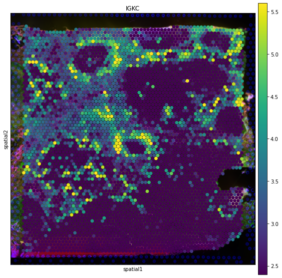
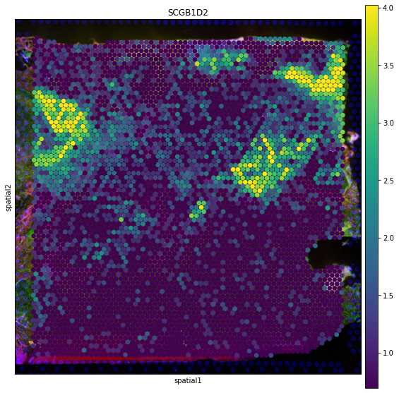
Finding differentially expressed genes

We find the differentially expressed (DE) genes across identified domains and show their expression patterns in spatial coordinates.

sc.tl.rank_genes_groups(adata, groupby='leiden', use_raw=False, layer='counts', method='t-test')

de_genes = pd.DataFrame(adata.uns['rank_genes_groups']['names']).iloc[:10,:]
de_genes

	0	1	2	3	4	5	6	7	8	9
0	MUC1	CXCL14	MT-CO2	CD74	SLC39A6	SCGB1D2	MALAT1	MGP	IGKC	IFI6
1	CXCL14	GALNT6	MT-ND1	APOE	ZNF703	SCGB2A2	CCDC80	H2AFJ	IGHG3	RPL30
2	TCEAL4	SPP1	MT-ND2	C1QB	CFB	CSTA	ANKRD12	SNHG25	IGHG4	RPL19
3	CCND1	MUC1	IGHG3	C1QA	BAMBI	S100G	IGKC	TFF3	IGLC2	NME2
4	TTLL12	COL1A2	IGKC	TIMP1	MUC5B	ADIRF	ATRX	ERLIN2	C3	HLA-B
5	KRT8	DNAJC1	MT-ND4	HLA-DRA	TMEM150C	MGP	SAMHD1	COPS9	IGHG1	NQO1
6	GALNT6	TCEAL4	IGLC2	FTL	RPS18	H2AFJ	FYB1	ZNF703	IGHA1	KRT19
7	KRT18	ATP9A	MT-ATP6	BGN	TNFSF10	HEBP1	HSP90B1	SLC9A3R1	C1QA	LGALS3BP
8	DEGS2	VEGFA	MT-ND5	HLA-DPB1	IGFBP5	FAM234B	CALD1	TOB1	IGLC1	BAMBI
9	AGR2	PRRC2C	MT-CO1	CTSD	XBP1	HLA-A	BOD1L1	ACTG1	JCHAIN	HLA-A

fig, axs = plt.subplots(figsize=(8, 8))

sc.pl.spatial(
    adata,
    img_key='hires',
    color=de_genes.iloc[0,5],
    layer='log1p',
    size=1.5,
    palette=sc.pl.palettes.default_102,
    legend_loc='right margin',
    vmin='p50',
    vmax='p99',
    show=False,
    ax=axs,
)

plt.tight_layout()

fig, axs = plt.subplots(figsize=(8, 8))

sc.pl.spatial(
    adata,
    img_key='hires',
    color=de_genes.iloc[0,8],
    layer='log1p',
    size=1.5,
    palette=sc.pl.palettes.default_102,
    legend_loc='right margin',
    vmin='p50',
    vmax='p99',
    show=False,
    ax=axs,
)

plt.tight_layout()